On Writing.
Score-based Diffusion Models (SBDMs)
•
SBDMs first progressively perturb the training data via a forward diffusion process.
•
And then learn to reverse this process to form a generative model of the unknown data distribution.
Forward Process
•
: training set with i.i.d. samples on .
•
: Intermediate distribution at time t.
•
: Forward diffusion process following SDEs.
: drift coefficient.
: diffusion coeffisient.
: infinitesimal positive timestep.
: standard Wiener process.
•
Denote : transition kernel from timestep 0 to t, which decided by and .
•
is usually an affine transformation w.r.t.
so that the is a linear Gaussian distribution
and can be sampled in one step. [Zhao et.al. 2021]
•
VP-SDE (Variance-preserving SDE)
Reverse Process
•
Reverse SDE by Anderson’s theorem: [Song et al. (2021)]
•
: standard Wiener process backward in time.
•
score-based model (approximate)
General Forms
: Gaussian Noise.
•
Forward Process:
•
Backward Process:
•
Choice of f, g, a, b:
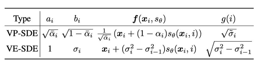
VP-SDE (DDPMs)
•
linear noise schedule:
⇒
VE-SDE (SGBMs)
•
Geometrical noise schedule:
⇒
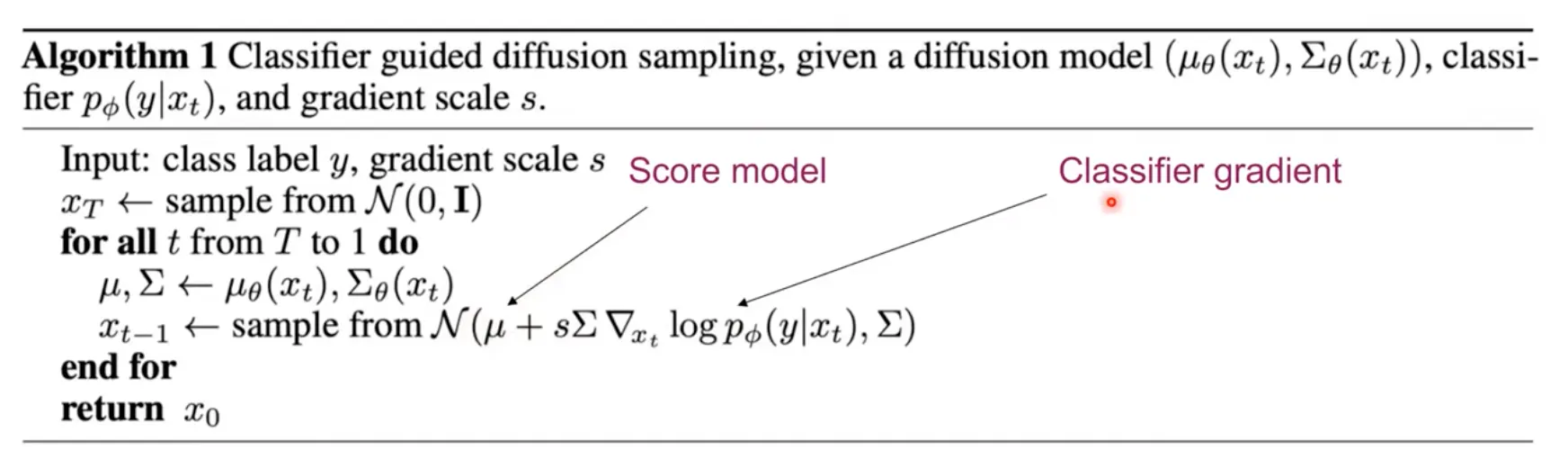
Controllable Generation
•
add guidance function to the score function:
Classifier Guidance
Unpaired I2I + SBDMs
•
Formulation Transfer Source image in source domain to target domain .
•
Goal Designing a distribution on target domain conditioned on an image to transfer.
ILVR (Choi. et al., 2021)
•
refine after each denoising step with a LPF .
EGSDE (Zhao et al., 2022)
•
design two energey-based guidance functions and follow cond. generation Song 2021.
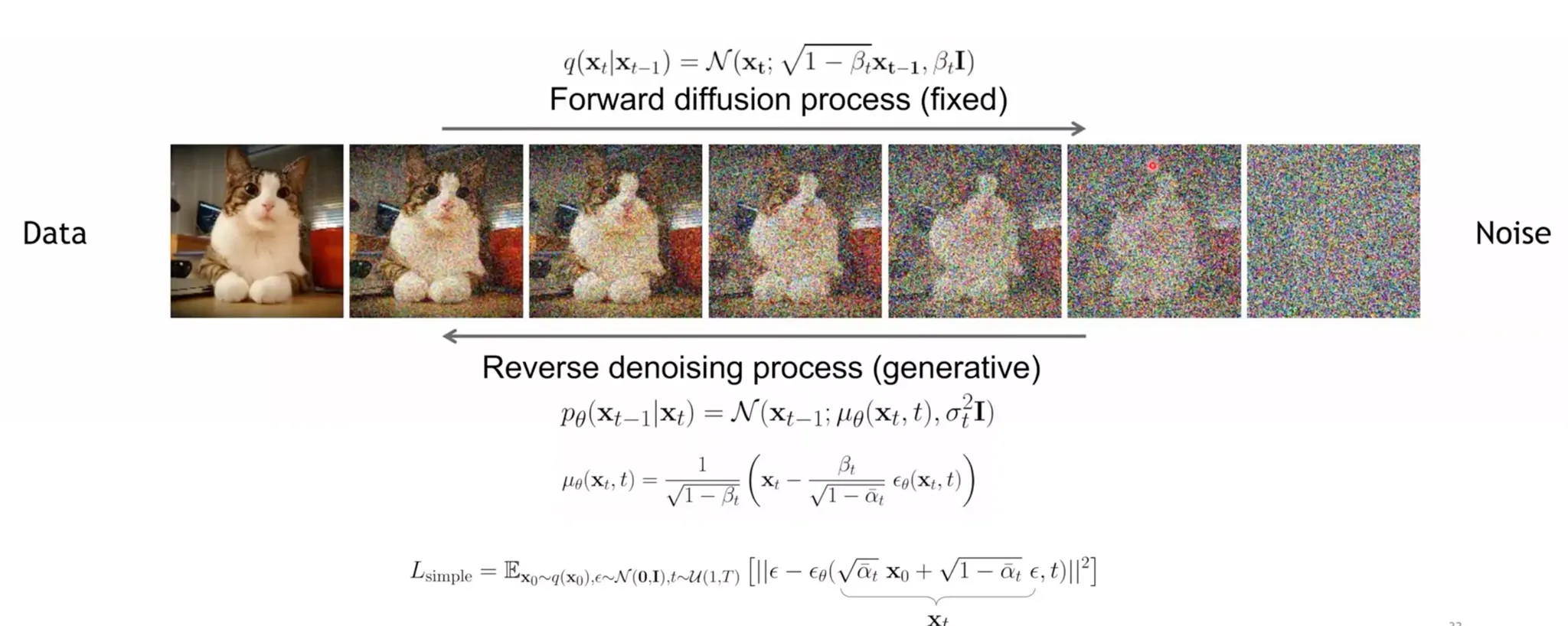
DDPM
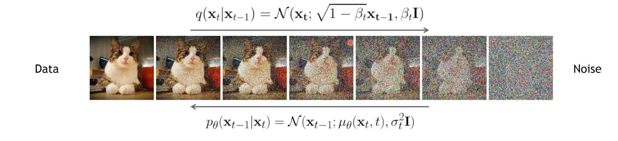
Forward Process
where and .
•
for sampling:
More Detailed Explain.
Reverse Process
Training
option #1 Predict directly as .
option #2 Predict the original sample , where
option #3 Predict the normal noise sample which has been added to the .
and hence

Loss: VAE to DDPM
Loss
Algorithm
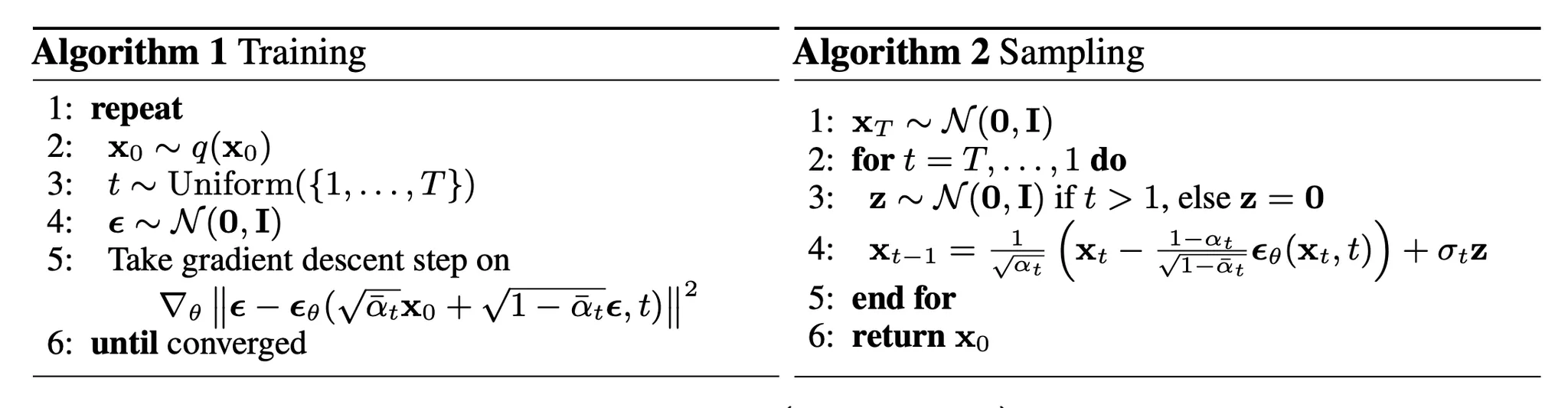
1.
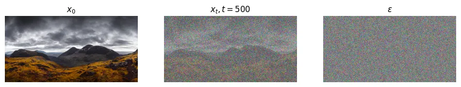
Forward Process: sample for .
a.
sample .
b.
sample . (가우시안 샘플링)
c.
compute . (Forward)
2.
Compute noise: using model with parameter .
3.
Minimize error: and by optimizing parameter .
Sampling
1.
Sample noise . (가우시안 샘플링)
2.
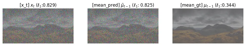
Predict the noise in the sample:
and approximate the mean of the process at .
3.
Next sample at is sampled from Gaussian distribution as:
...until is reached, in which case only the mean is extracted as output.
•
better sample quality at fewer steps.
•
Allows for deterministic matching between the starting noise and the generated sample .
•
Perform worse that DDPM for large numbers of steps ( e.g. 1000).
Noise Schedule
Visualization
•
: Low Frequency 혹은 High Frequency를 만들 것인지 네트워크에게 알려주는 역할
Summary
DDIM: Sampling Faster. Non-Markovian process.
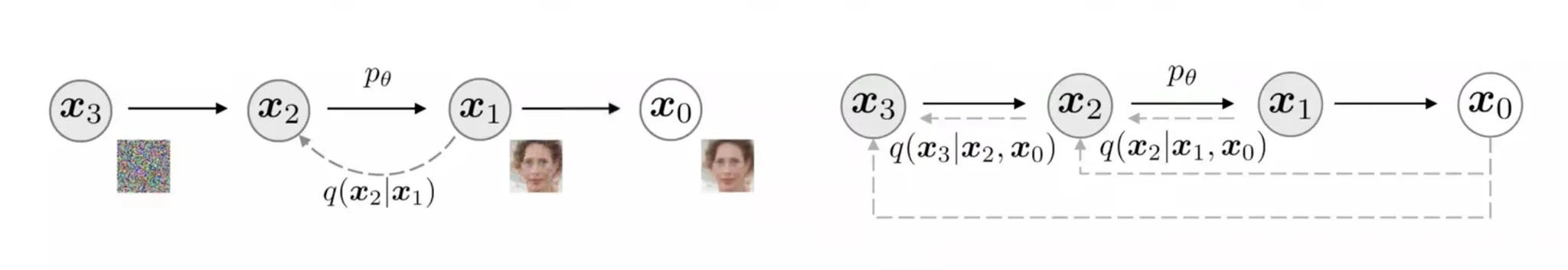
•
DDPM (Markovian) → DDIM (Non-Markovian).
•
다 같고, 샘플링만 다르다.
Details
From DDPM equation (1) at ,
which yields,
based on specific measured at the previous step ,
if =0, deterministic. (noise:image=1:1 matching)
Generally, is set to:
new parameter to comtrol the magnitude of the stochastic component:
•
: appears to be particularly beneficial when fewer steps of the reverse process are applied and that specific type of process is known as DDIM.
•
: DDPM.
So, how can the reverse chain be navigated in the reverse direction?•
First, a sequence of fewer steps is defined as a subset of the original temporal steps of the forward process. Sampling is then based on (8).
DDIM: Sampling
1.
predict .
2.
Compute the direction towards current .
3.
(if not DDIM) inject noise for stochastic functionality.
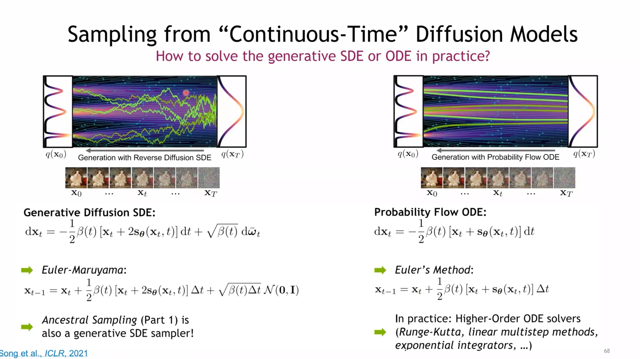
SBDMs
Visualization
미분방정식처럼 생겼지? Solve with SDE.
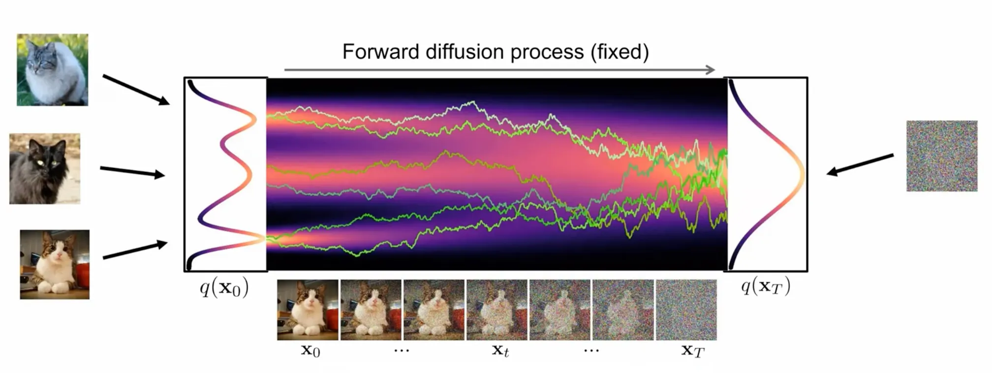
Forward SDE:
Reverse SDE (Anderson 1982)
•
To Solve Reverse SDE, How to get score function?
option #1 Naive way: NN으로 score func. 학습.
⇒ But score of marginal diffused density is not tractable!
중간 timestep을 알 수 없어서 학습이 안됨.
option #2 Given .
•
Denoised score matching:
⇒ After expectation,
Details
•
Consider reverse generative diffusion SDE:
•
In distribution equivalent to “Probability Flow ODE”:
•
initializing