STEGO: Unsupervised Semantic Segmentation by Distilling Feature Correspondences

Task: Unsupervised Semantic Segmentation
Intro & Overview
•
Semantic segmentation은 pixel-level의 classification이며 이것은 image-level의 corpora나 ontology등의 시스템이 배경으로 깔려있다.
◦
Problem Expensive Annotation (박스 대비 100x 비용)
◦
Problem Complex Domain에서 잘못된 Annotation 가능성
•
이를 해결하기 위해, Weekly supervised 방식이 제안되었다.
•
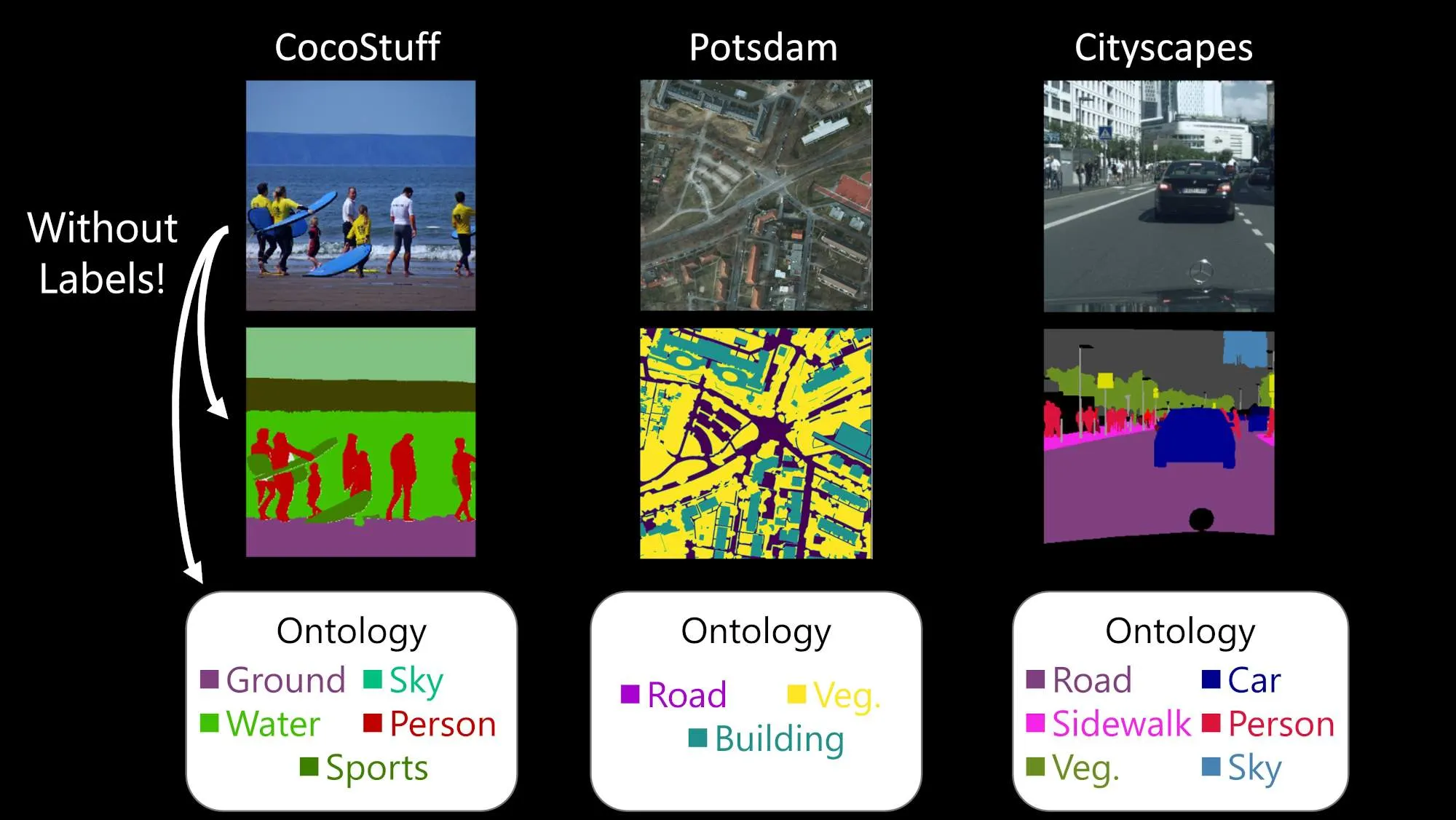
Unsupervised semantic segmentation은 이미지 내부의 corpora에서 어떠한 annotation 없이, semantically meaningful한 카테고리를 찾고 localize 하는 것을 목표로 합니다.
•
이를 위해서 이미지 내부의 모든 픽셀은 semantically meaningful하고 compact enough한 클러스터를 형성해야 합니다.
Related Works
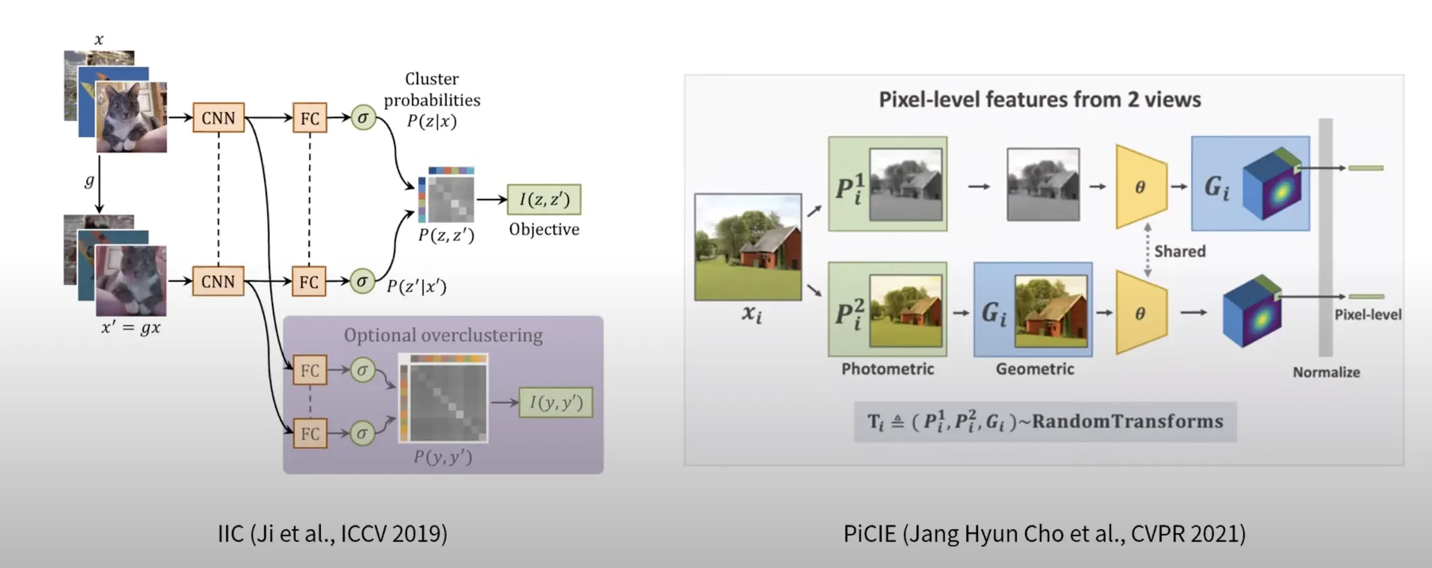
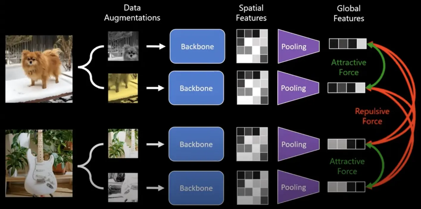
IIC (Ji et al. ICCV 2019)
•
같은 영상에 다른 Pertubation을 주고 둘 간의 Mutual information을 maximize하는 방식을 제안
PiCIE (Jang Hyun Cho, CVPR 2021)
•
이미지에 variance (geometric/photometric) 을 주고
이에 대한 feature를 k-means로 clusturing한 후 (Pseudo label)
그 결과를 cross-entropy로 학습하는 접근 방법
Motivation
•
CNN 기반의 Backbone → Transformer 기반의 Backbone
Methodology
Idea Deep features connect objects across the Image
STEGO의 순서 (영어가 더 명쾌해서 영어로 !)
1.
Distills pretrained unsupervised visual features into semantic clusters using a novel contrastive loss
2.
Agnostic to feature backbone
3.
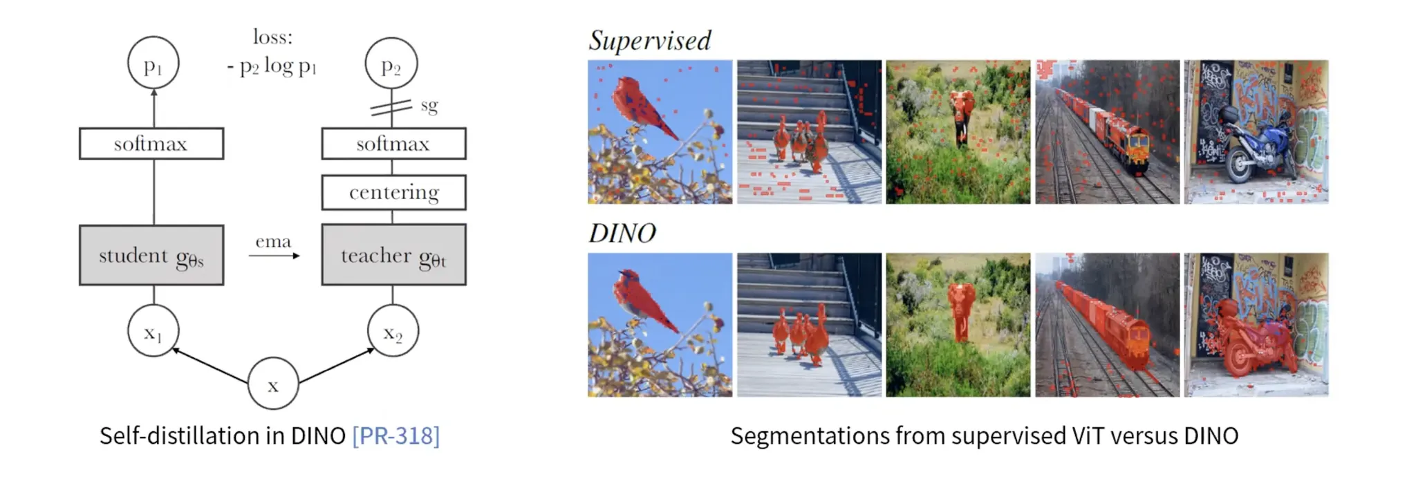
Focuses on DINO’s embedding because of their quality
•
Training Objective: Obtain and distill feature correspondence
Feature Correspondence
가 두 이미지의 텐서라면,
(c는 채널, hw 와 ij는 spatial dimension)
•
Cosine Similarity를 Channel-wise로 구한 후 summation 한 것입니다.
•
만약 이면 self-correspondence 가 됩니다.

credit: https://mhamilton.net/stego.html
•
위 그림에서 땅에 대한 query point는 땅을 segmentation 하는 결과를 얻고
하늘에 대한 query point는 하늘을 segmentation 하는 것과 유사한 결과를 얻는 것을 볼 수 있습니다.
여기서 저자는 self-correspondence를 조금 더 파보기로 합니다.
Self-correspondence
GT mask label 라고 할 때, (C는 possible class)
co-occurence tensor는 다음과 같이 구성됩니다.
•
각 pixel마다 cluster label이 할당되었을 때,
같은 픽셀끼리 같으면 1, 원래 같은 픽셀인데 다르게 나왔으면 0이라는 notation을 만듭니다.
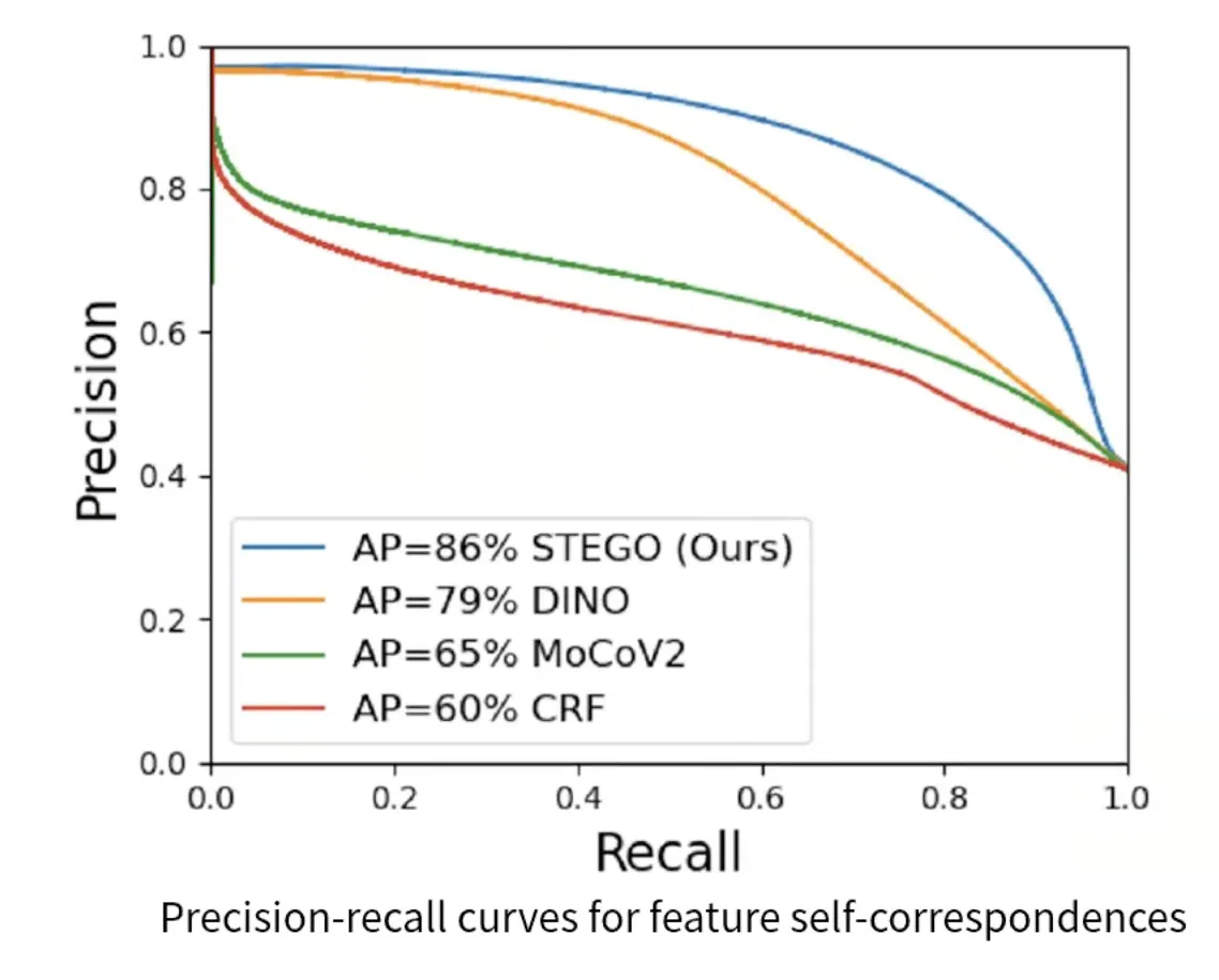
→ How well dows F proedict L?
•
F: probability logit
•
L: ground Truth
L이 일치하는지 보는 커브
→ DINO, MoCo보다 Precision이 매우 개선되었습니다.
⇒ 원본과 copy본 간에 correspondence가 높은 precision으로 보장이 된다면 이를 semantic segmentation prediction으로 활용할 수 있겠다는 근거로 활용하고 있습니다.
Distilling Feautre Correspondences
•
지금까지는 label의 co-occorance를 활용하는 단계는
semantic segmentation으로 활용될 수 있는 가능성을 보기 위한 단계였습니다.
•
어떻게하면 Quality Segmentation Task를 할 수 있을까요?
Feature correspondence와 segmentation correspondence간 multiplication을 적용한다!
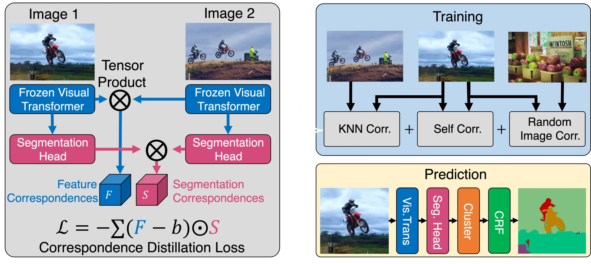
High-level overview of the STEGO architecture at train and prediction steps.
1.
Let Feature Backbone
that maps an image to a feature tensor (e.g. DINO backbone) → FROZEN
2.
(중요) Focus only on light-weight semgentation head
that maps the feature space to a code space of dimension K ( K < C , K는 code의 수)
3.
a pair of images and ,
→ feature tensor and ,
→ segmentation features and
⇒ Compute 1) a feature correlation tensor F from and ,
2) a segmentation correlation tensor S from and .
Correspondence Distillation Loss
학습 방향:
feature tensor 와 가 커플링이 뚜렷하게 있으면,
같은방향으로 push 하도록 segmentation head를 학습
Simple element-wise multiplication of the tensor F and S:
•
: hyper-paramter, collapse를 방지하기 위해 negative pressure (impherically)
•
zero-clamp: for stable optimization:
•
Spatial Centering: for balanced optimization:
작은 물체를 잘 segmentation 하기 위해, mean을 계속 밀어주면 개선이 된다고 합니다.
Final correspondance distillation loss:
STEGO’s full loss
•
위에서 봤던 3가지 task로 확장한 최종 Loss Function.
•
Feature의 GAP 결과에 대하여 KNN을 수행하고,
그것에 대한 cosine similarity lookup 테이블을 만들어 sampling할 때 활용했습니다.
•
Robust to small objects: Five-cropping, Clustering, CRF 와 같은 테크닉을 많이 사용했습니다.
Experimental Results
•
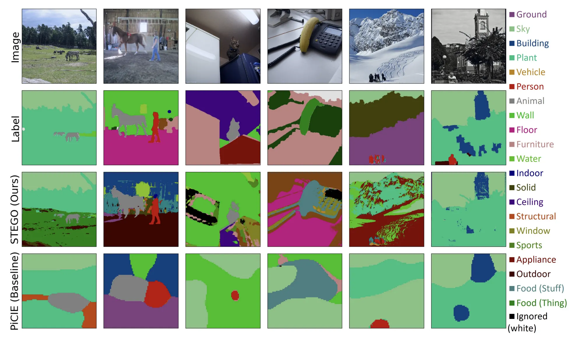
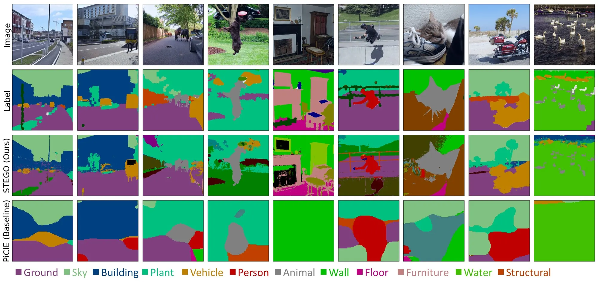
STEGO는 fine-grained를 굉장히 정확히 표현합니다.
•
PiCIE와는 비교가 안됩니다.
•
•
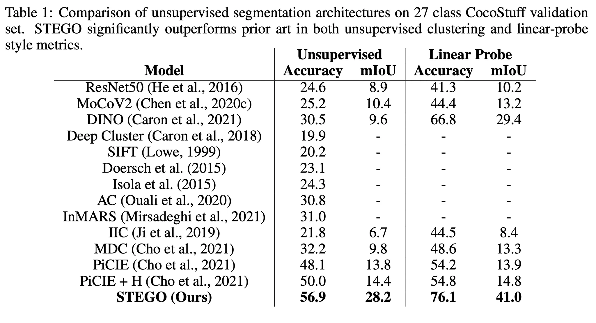
Metrics:
◦
Accuracy는 헝가리안 matching algorithm을 사용해서 cluster와 GT class간 mapping을 해준 후 accuracy를 측정했습니다.
◦
mIoU는 main task에 해당합니다.
◦
Linear Probe는 labeled data를 이용해 finetuning 을 거쳐 결과를 보는 것입니다.
•
기존의 결과에 비해 굉장히 큰 폭으로 결과가 상승했음을 볼 수 있습니다.
•
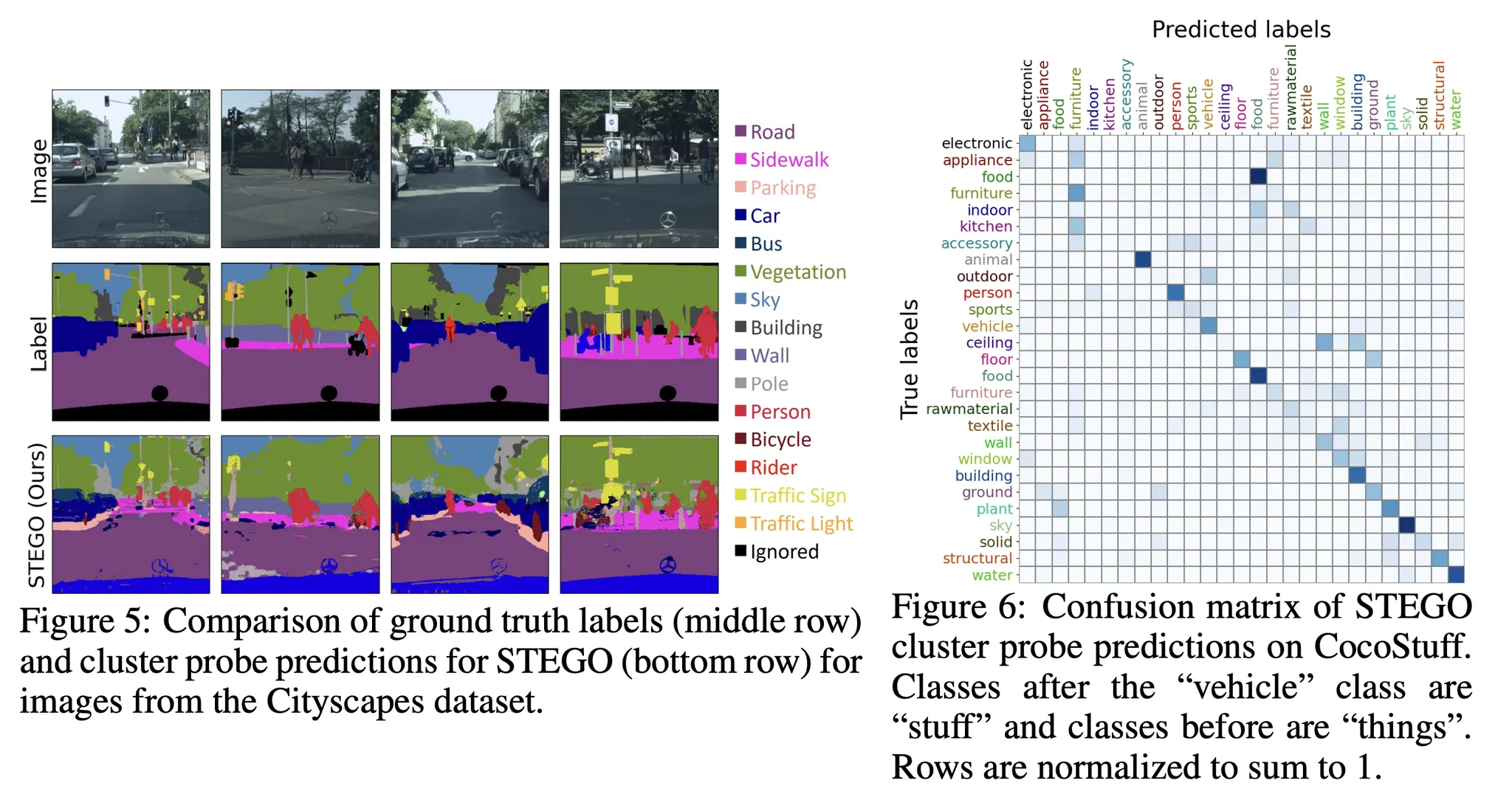
Confusion중 튀는 점 하나는 같은 food 카테고리입니다.
저자들은 이런 결과를 보고 label system 에 대한 의구심을 제기합니다.
•
즉, 자신의 STEGO는 clustering은 잘 되었으나, True label의 ontology가 반드시 진리가 아니기 때문에 저런 confusion matrix가 나왔다는 것이죠. 이렇게 강하게 소신을 밝힌다는 것이 재밌습니다.
•
그 근거로써 linear probe로 finetuning을 했을 때 결과가 매우 좋아진다라는 점을 들고 있습니다.
Ablation Study
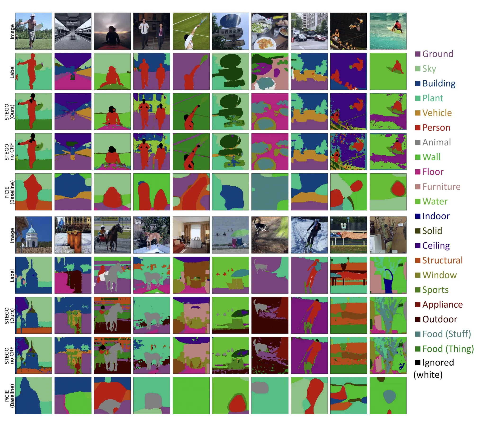
Additional unsupervised semantic segmentation predictions on the CocoStuff 27 class segmentation challenge using STEGO (Ours) and the prior state of the art, PiCIE. Images are not curated.
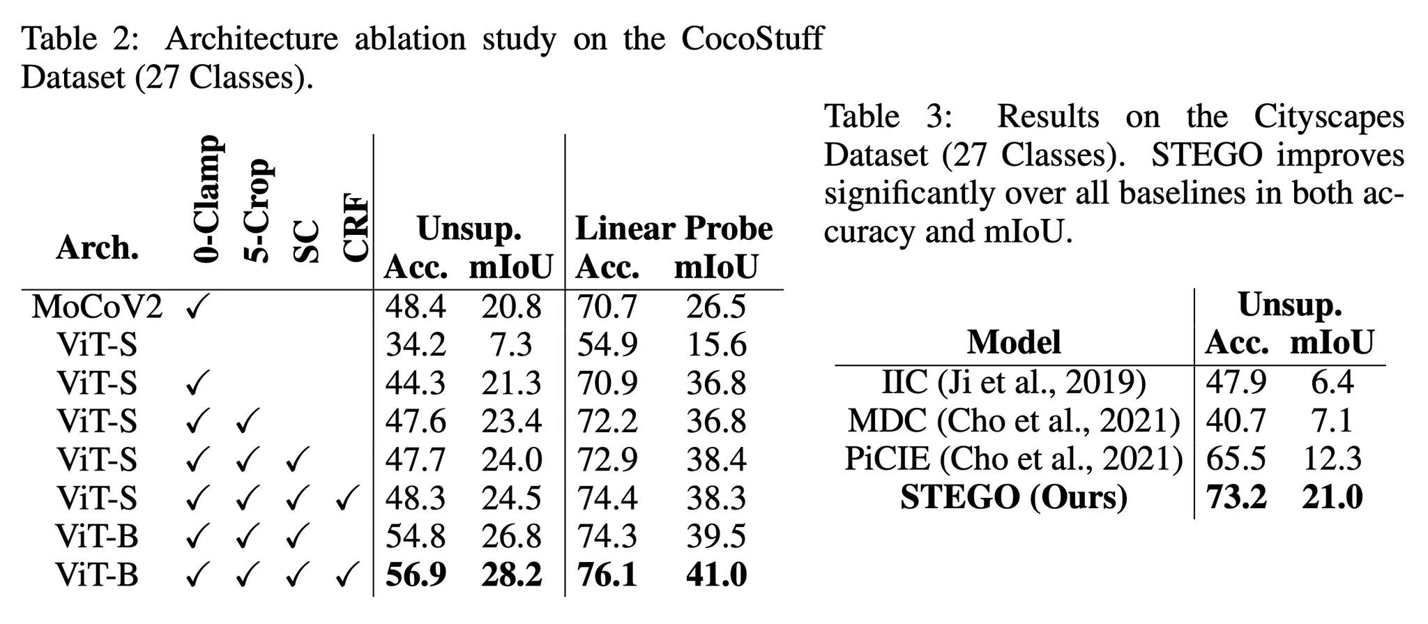
•
ViT-Small 베이스를 사용하면 0-clamp와 5-crops를 도입했을 때 moco와 비슷한 수준까지 올라오고,
SC와 CRF까지 넣으면 MoCo를 능가한 성능이 나옵니다.
•
ViT-Big을 베이스로 사용하면 성능이 바로 올라옵니다.